Adaptive Empirical Local Patches
The preparation of empirical local patches involved the following steps:
- Data transformation: To calculate a semi-variogram, the data were transformed into a normally distributed, seasonality-removed time series.
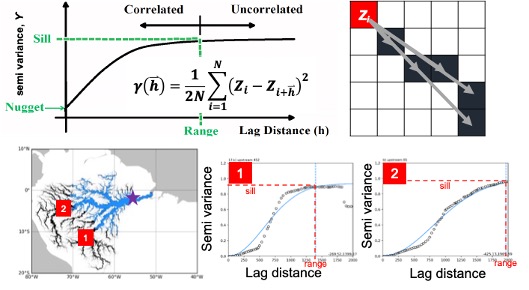
- Semi-variogram analysis: A semi-variogram summarizes the spatial dependence structure by a one-dimensional spatially averaged semi-variance.
Data Transform
WSE was simulated using the CaMa-Flood hydrodynamic model. Remove the linear trend from the simulated WSE. Remove seasonality from the detrended time series. Standardize by dividing by the standard deviation.
![]()
Semi-Variogram Analysis
A semi-variogram was calculated for each pixel using the average squared difference between all pairs of values separated by the spatial distance lag.
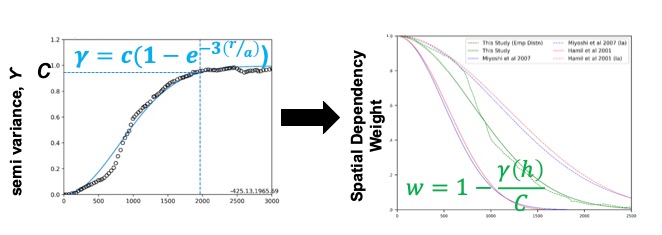
Preparing Empirical Local Patch
Semi-variogram fitting was conducted for each upstream location. Spatial dependency weights were calculated for each tributary corresponding to each target pixel. A threshold of 0.6 was defined to delineate the extent of the empirical local patch. Convert semi-variance data into an empirical weighting function Inverting standardized semi-variances using the sill value (C)
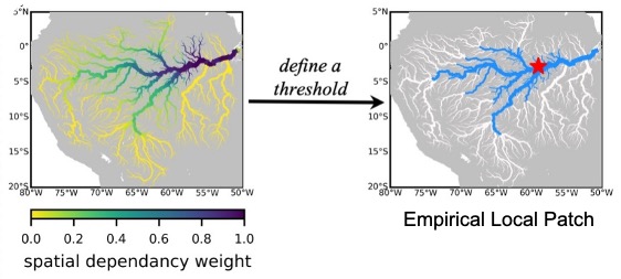
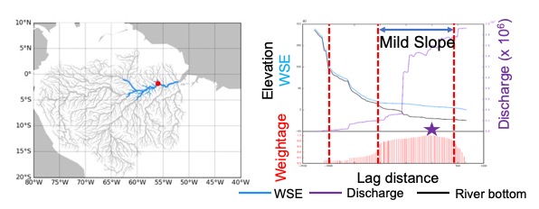
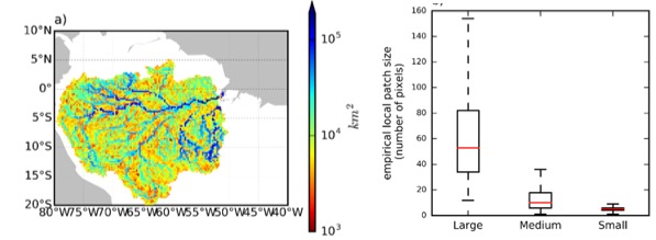
Characteristics Empirical Local Patch
Empirical Local Patch: follow river hydrodynamics, consider significant correlation areas, remove nonsignificant correlations, remove error covariance. The size of each empirical local patch is determined by the river hydrodynamics. The empirical local patches created for different river pixels vary in size. Small rivers have relatively smaller local patches, while large rivers have larger ones.